Planning of Water and Hydropower Intake Structures (GTZ, 1989, 122 p.) 1. Hydrological bases 1.1 Presentation of the problem 1.2 Determination of the available water supply 1.3 Suspended matter and bed load

Planning of Water and Hydropower Intake Structures (GTZ, 1989, 122 p.)

1. Hydrological bases

1.1 Presentation of the problem

Intake structures on channels are intended to divert a certain amount of water Q from the channel for various purposes of use (irrigation, potable water supply, hydroelectric power). It must be possible for both the diverted water and the remaining supply to be evacuated without damage being caused.

To perform this task, constructional measures must be taken in and on the channel, and it is necessary to design the intake structures hydraulically and to determine the necessary amount of water to be drawn off. For this purpose, the basic hydrological data must be known or the

- precipitation and
- discharges

The methods and procedures described in this planning guide have been deliberately simplified but they offer a comprehensive representation of the hydrological processes of a catchment area which is sufficiently exact for planning purposes. The methods described here are, however, subject to the following conditions:

- The channel to be considered carries water all the year round.
- The discharge is exclusively formed by - precipitation in the form of rain.
- The catchment areas are smaller than 1,000 m²,
- The discharge behaviour of the river is not influenced by a retention reservoir.

To understand the discharge behaviour of a river, it is necessary to know the water cycle; this is described in Fig. 1.

All the water available in the catchment area such as surface runoff, intermediate runoff, groundwater runoff and air moisture results from precipitation. In each catchment area, however, only a part of the precipitation runs off, the so-called effective precipitation. After a precipitation event, this precipitation runs off in the form of

- surface runoff and
- intermediate runoff.

The residual precipitation, the greatest part of which does not run off, is referred to as loss and is subdivided into the following components:

- interception and trough losses,
- evaporation,
- increase in soil moisture and infiltration.

Besides the direct runoff from precipitation events, in most catchment areas, the runoffs are also supplied from the groundwater during periods with low precipitation. This is why there is a basic runoff which ensures that the rivers described here carry water all the year round.

For a short period of time T immediately after a precipitation event, the following water regime equation is valid:

N = A + V + R

where N = precipitation above the catchment area during the period of time considered T, A = runoff during T, V = evaporation above the catchment area during T, R = retention in the catchment area during T (= interception, infiltration, etc.).

Fig. 1: Simplified representation of the water cycle

When the above-mentioned hydrological quantities are related to the precipitation area AEO, the following components which are important in applied hydrology are obtained:

h_N = N / A_E0 = height of precipitation above A _E0 during T in mm

h_A =A / A_E0 = runoff rate of the A_E0 during T in mm

h_V = V / A_E0 = evaporation height in the A_E0 during T in mm

h_R = R / A_E0 = retention rate in the A_E0 during T in mm

Hence the following water regime equation is valid:

h_N = h_A + h_V + h_R (in mm)

Another important characteristic of the runoff behaviour of a catchment area is the runoff coefficient y which gives the ratio of the effective precipitation (= precipitation which might form runoff) to the total precipitation:

y = h_A / h_N

The runoff coefficient of a catchment area varies in the course of a hydrological year, as it does not depend only upon area-specific factors such as

- topography,

- geology,
- vegetation,

but also upon event-specific factors such as

- soil moisture before precipitation event,
- season,
- duration of precipitation,
- height of precipitation,
- development and seal coat.

1.2 Determination of the available water supply

The rain gauge can measure only the total precipitation falling within a period of reading. Rain gauges are therefore also referred to as totalizers. The data can be evaluated only as the precipitation sum for certain periods of time (day, month, year). It is not possible to measure an individual event as the observation staff does not carry out the reading after each precipitation event but at a certain time (ea. each morning at 8 a.m.).

On the other hand, the rain recorder records precipitation events on a recording roll or other recording media, depending upon the make. The most usual instruments work on the float or tipping bucket principle (cf. Fig. 2). If maintenance is carried out regularly and the recorder is in good working order, each individual precipitation event can be evaluated. From the records of the recording roll, the duration of precipitation TN in h, the height of precipitation hN in mm and the intensity of precipitation iN in mm/in can be read or determined (cf. Fig. 2).

The quality of the data from precipitation records is dependent upon the maintenance of the instruments, the ability of the observation staff to read the data correctly, and, above all, upon the place of installation. If possible, the rain gauge should be installed in a place where it is possible to record precipitations which are more or less representative of a certain part of the catchment area.

Type of region	Catchment surface per station (km²)
I. flat terrain, temperate to tropical zones	600-900
II. hilly terrain	100-250
III. mountainous terrain with varying distribution of precipitation	25

Table 1: Minimum density of a rain gauge network

The total number of rain gauges installed in a catchrnent area decisively influences the exact, representative determination of the total precipitation (cf. section 1.2.3). The number of gauges to be installed depends upon the degree of homogeneity of the distribution of precipitation above the catchment area and upon the topography of the latter.

The lowest density of a rain gauge network according to the WMO rules can be seen in Table 1.

The measuring instrument must be so installed in the terrain that buildings, trees, etc., and the wind do not falsify the precipitation measurement.

All the above-mentioned criteria must be taken into consideration during the collection of data and particularly in the evaluation.

The informational content of the precipitation data depends not only upon the quality of the data recording in situ but also upon the length of the observation period. For the statistical evaluation of the precipitation events, observation series over a period of at least 20 years are necessary. If possible, the observation series should not be interrupted.

Detailed information regarding the construction, operation and cost of precipitation measurement stations is given in the literature [2] and Annex 1.

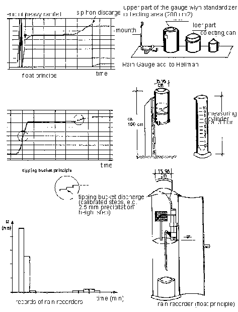
Fig. 2: Precipitation measuring instruments and precipitation recording

1.2.1.2 Discharges and water levels

The measurement of the discharge is in most cases carried out at gauging stations which are installed at the outlets of individual partial catchment areas or at the outlet of a larger catchment area.

A stationary gauging station comprises a gauge to record the water levels and a device for measuring the flow velocity v in m/s. At a cross-section of flow A in m² which is known or is to be determined and at the measured mean flow velocity vm in m/s, this indirect method allows the discharge Q in m³/s to be determined as follows:

Q = A x V_m (in m³/s).

An exact method for determining the flow velocity is the current meter measurement. On the basis of the number of revolutions of a verified current meter, the mean flow velocity v_m is determined by the method explained in section 1.2.2.

A very imprecise but relatively simple and rapid method is the velocity measurement using floats. By this method the mean flow velocity vm is determined with floats or flotsam and jetsam. It gives a rough knowledge of the discharge conditions, particularly at the cross-sections where an intake structure is planned and discharge measurements have not yet been carried out.

Besides this indirect method, the discharge on small streams can also be directly measured with the aid of a simple wooden weir (cf. section 1.2.2).

During a discharge measurement, the water depth h pertaining to the discharge is also recorded. For this purpose the water-level gauge is used.

Water-level gauges are used in the form of staff gauges and water-level recorders. The staff gauge should be so arranged that the gauge observer can read the staff at any water level. Readings are carried out at certain times (e.g. 8 a.m., 5 p.m., etc.). The observer enters the value in the field book. During a discharge measurement the respective water level should also be read.

A recording gauge continuously registers the water level. The values are usually recorded on a recording roll. Besides a waterlevel recorder, a staff gauge should always be used for checks.

Fig. 3: Water level/discharge radiation (discharge curve) of a channel cross-section

If the discharge measurement is carried out for the range from the lowest discharge to peak discharge, and if for every different discharge value determined the corresponding water level is entered into a system of coordinates, the discharge curve characteristic of a certain discharge cross-section is obtained. With this discharge curve it is possible to read the discharge corresponding to any water level (water depth h) which can be determined relatively rapidly and simply with a water-level gauge (cf. Fig. 3).

This procedure is widely used for economic reasons, as a calibrated discharge curve allows the relatively expensive discharge measurements to be dispensed with. Only one record with a water-level gauge is necessary at the measuring station. This method can, however, be applied only at cross-sections of flow which are not subject to strong seasonal changes of the river bottom and the banks by denudation or alluvial deposits, i.e. the cross-section of flow must be stable.

If, however, the cross-section of flow is unstable, i.e. if the river bottom or the banks are changed by erosion or alluvial deposits during the periods of lowest and peak discharges and if a more suitable site for a discharge measuring station cannot be found, the discharge must be measured continuously and the discharge curve permanently checked by measurements and, if necessary, corrected.

The quality of the discharge measurements and, thus, of the discharge data chiefly depends upon the execution of the discharge measurement. An accurate discharge measurement is possible only with experienced staff who are aware of the numerous interrelations and their influence upon the measurement. This is why the kind of data collection and its execution should, if possible, be taken into account when the data are analysed.

1.2.2 Performance of simple discharge measurements

1.2.2.1 Indirect measurement

In indirect measurement, the discharge at a known cross-sectional area A is determined via the mean Dow velocity vm as follows:

Q = A · V_m (in m³/s).

- Current meter measurement
As the velocity is irregularly distributed in the cross-section of the river, it must be measured in several vertical lines for measurement at different water depths. The velocity at a point of measurement is obtained from the number of revolutions of the current meter during the time of measurement which must not be less than 20 seconds.

The equation calibrated for each current meter

v = n · a + b (in m/s)

where v = determined flow velocity, n = number of revolutions per unit of time, a, b = calibrated parameters (as given by the instrument manufacturer) allows the present flow velocity at the point of measurement to be determined. When the individual velocity values of the vertical line for measurement are plotted, the velocity profile of this line is obtained (cf. Fig. 4). The velocity area is evaluated by planimetering or by summing up the individual areas:

f_vm = (h₁ · (v₀ + v₁) / 2) + (h₂ · (v₁ + v₂) / 2) + . . . etc.

With the simplified and most rapid method, only two points of measurements are selected on the vertical line for measurement at 2055 and 8056 of the water depth. The mean velocity results from the arithmetic mean of the two measurement values. The value of the velocity area is obtained by multiplication of the mean velocity by the total water depth h on this vertical line.
When the values of the individual velocity areas are plotted above the corresponding vertical line, the total discharge Q in m³/s is obtained by planimetering or summing up these individual partial areas as follows (cf. Fig. 4):

Fig. 4: Determination of the mean flow velocity in a river cross-section

Q = ((f_v0 + f_vI)· b₁ / 2) + ((f_vI + f_v|I) · b₂ / 2 + . . .

To perform these current meter measurements, the current meter can either be fixed to a rod or suspended with a weight and a float from a wire rope (Fig. 5). In the latter case, a relatively expensive cable crane installation is necessary. The advantage of the velocity measurement with the current meter lies in the simultaneous determination of the wetted area, as the water depth at a vertical line for measurement can be directly measured at the same time with the rod or the cable crane installation.

Fig. 5: Discharge measuring instruments for current meter measurement

The criteria for the use of a current meter are as follows:
current meter on a rod: max. flow velocity < 2.00 m/s; max. water depth < 1.50 m
current meter on a float with weight: max. flow velocity 5 m/s.

For flow velocities > 5 m/s, the discharge should be determined by the velocity measurement using floats as described below.

- Velocity measurement using floats
For the determination of the discharge with floats, the wetted area must be known or determined. In the case of small rivers, this is possible by measuring the water depth on several vertical lines for measurement with rods. The velocity is approximately determined with floats (bottles, wood, cork). If possible, the measurement section should be so long that the floats drift for about twenty seconds. Moreover, it should be straight without obstacles such as trees, ashlars, small islands or rapids, so that a more or less uniform velocity is ensured.

The individual velocity values measured

v_i = s / t - (in m/s)

with s = length of measurement section in m, t = drifting time of the float

are higher at the surface than the mean velocity values and must therefore be reduced
with a correction factor of 0.8 to

v_i* = 0.8 · v_i (in m/s).

From the mean value of all measured partial velocities of each float used, the mean velocity v_m is determined with which the instantaneous discharge

Q = A · V_m (in m³/s)

can be calculated.

1.2.2.2 Direct measurement

On small and medium-scale rivers, structures in the form of measuring weirs with rectangular overfall which are artificially arranged in the channel cross-section are suitable for discharge measurement (cf. Fig. 6). The rate of discharge is determined with the aid of the weir head h to be read. For the rectangular cross-section the calculation is made using the following formula:

rectangular weir:

(in m³/s)

where b = width of weir in m, w = height of weir body in m, h_e = h + 0.0011 m (= substitute weir head according to Rehbock [14]).

The discharge measurement must be carried out under the following conditions:

b ³ h
w ³ 0.3m
0.1 < h < 0.8m
Q_min = 40 l/s
1 = 4 h.

Furthermore, the wooden weir must be tight. All edges of the weir must be sharp; this is achieved by an arris sloping towards the downstream side (cf. Detail A in Fig. 6). It is best to use a metal rail for this purpose.

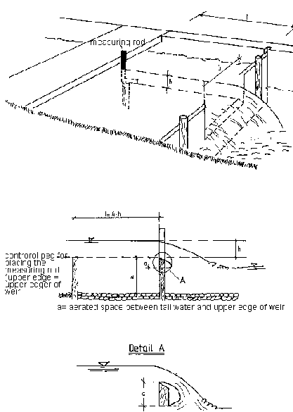
Fig. 6: Discharge measurement with a rectangular weir

(1) Earth canals	ks
	Solid material, smooth	60
	Sand with some clay or broken rock	50
	Bottom of sand and gravel, with paved slopes	45-50
	Fine gravel, about 10/20/30 mm	45
	Medium gravel, about 20/40/60 mm	40
	Coarse gravel, about 50/100/150 mm	35
	Cloddy loam	30
	Lined with coarse stones	25-30
	Sand, loam or gravel, strongly overgrown	20-25
(2) Rock canals
	Medium coarse rock muck	25-30
	Rock muck from careful blasting	20-25
	Very coarse rock muck, great irregularities	15-20
(3) Masonry canals
	Brickwork, bricks, also clinker, well pointed	80
	Ashlars	70-80
	Thorough rubble masonry	70
	Normal masonry	60
	Normal (good) rubble masonry, hewn stones	60
	Coarse rubble masonry, stones only coarsely hewn	50
	Rubble walls, paved slopes with bottom of sand and gravel	45-50
(4) Concrete canals
	Smooth cement finish	100
	Concrete when steel formwork is used	90-100
	Fair-faced plaster	90-95
	Smoothed concrete	90
	Good formwork, smooth undamaged cement plaster,
	smooth concrete with high cement content	80-90
	Concrete when wood formwork is used, unplastered	65-70
	Tamped concrete with smooth surface	60-65
	Concrete shells with 150-200kg cement/m²,according to age and design	50-60
	Coarse concrete lining	55
	Irregular concrete surfaces	50
(5) Wooden channels
	New, smooth channels	95
	Planed, well-joined boards	90
	Unplaned boards	80
	Older wooden channels	65-70
(6) Plate channels
	Smooth pipes with flush rivets	90-95
	New cast-iron pipes	90
	Riveted pipes, rivets not flush, several times
	overlapped on the circumference	65-70
(7) Other linings
	Rolled mastic asphalt lining of the works canals	70-75
(8) Natural water courses
	Natural river bed with solid bottom, without irregularities	40-42
	Natural river bed with moderate bed load	33-38
	Natural river bed, weedy	30-35
	Natural river bed with rubble and irregularities	30
	Natural river bed, rich in coarse bed load	28-30
	Foreland, according to vegetation	20-25
	Torrent with coarse rubble (head-sized stones), bed load at rest	25-28
	Torrent with coarse rubble, bed load in motion	19-22

Table 2: Strickler coefficients k_S in the Manning-Strickler formula

1.2.2.3 Discharge calculation

Besides the determination of the discharge with the aid of measuring instruments, it is also possible to calculate the discharge theoretically using the Manning formula for open channels:

v = k_S I^1/2 r_hy^2/3 (in m/s)

where

k_S = coefficient of roughness in m^1/3/s,
I = bottomslope,
r_hy = hydraulic radius in m = F / 1_u = wetted area/wetted perimeter = in m²/m
r_hy and I must be determined in the terrain, whereas the coefficient of roughness can be taken from tables (cf. Table 2). When the velocity is known, the discharge can be calculated:

Q = A V_m (in m³ /s).

1.2.2.4 Estimate of rates of discharge

When discharge measuring stations which have been used for many years are not situated in places which are of interest in the construction of an intake structure or when no discharge values at all are available, the rates of discharge can be estimated or transferred.

If discharge data are lacking, a simple estimate is possible with the aid of the discharge coefficient y. When the discharge coefficient is multiplied by the amount of precipitation N, the estimated rate of discharge V_Q is obtained:

V_Q = y N (in m³).

According to the precipitation sum value, this estimate can relate to daily, monthly or annual rates of discharge. Attention should be paid to the event and area-specific dependence of the discharge coefficient (cf. also section 1.1).
If discharge data are available for neighbouring stations of the catchrnent area (cf. Fig. 7), the discharges Q_X at the place x can be transferred from the known discharges. For catchment areas which do not vary too much in nature and size, the discharge can be determined according to the proportionality of the catchment area surfaces A_E0:

Q_X = Q₁ A_X/A₁

If a short series of discharge data is available for the place of interest, a correlation with the discharge data of any other measuring station in the neighbourhood can be sought. It is usual to use linear correlations of the monthly and annual mean values. If there is a good correlation between two stations, the measurements over a period of many years can be used for the place of interest. Detailed information is given in [4]. It should be taken into account that the transfer formulas for peak and lowest discharge are usually different.

1.2.3 Simple data evaluation

1.2.3.1 Precipitation

If precipitation data acquired over several years of observation are available for several stations of a catchment area, the periods of observation of each station should be entered in a bar chart so that these data can be evaluated and analysed (cf. Fig. 8).
The orientation frame is extremely helpful when the available precipitation data are compared and analysed with a view to finding certain interrelations between the individual stations.

Fig. 7: Estimate of discharge

Furthermore, the precipitation data available can be checked either for irregularities in the data recording or for a change in the precipitation behaviour of a region if the two stations are situated at a great distance from each other. For this purpose, the accumulated data of two neighbouring stations are plotted against each other (cf. Fig. 9).

Fig. 8: Possibilities of the precipitation analysis

Figure

m	m/n+1	N(mm)	m	m/n+1	N(rnm)
1	0.033	21.4	14	0.536	26.5
2	0.077	22.0	15	0.577	27.6
3	0.115	20.5	16	0.615	29.1
4	0.154	23.3	17	0.654	30.0
5	0.192	23.6	18	0.692	30.0
6	0.231	23.8	19	0.731	30.1
7	0.269	24.1	20	0.769	32.0
8	0.303	24.3	21	0.807	33.8
9	0.345	24A	22	0.845	35.9
10	0.305	24.6	23	0.885	33.2
11	0.423	24.7	24	0.923	40.0
12	0.462	24.9	25	0.962	45.3
13	0.500	25.5

n = number of events, m = event number (1 = smallest event), N = precipitation (in mm), here: maximum annual 1-hour precipitation, period of observation: 25 years.

Fig. 9: Determination of the probability that definite precipitations are not reached. Source: [1]

Trends and changes in the slope of the curves or straight lines can be due to a change in the method of data collection or to a change in the precipitation behaviour of the region.
If the precipitation records of a station are in the form of recording strips for a prolonged period of observation (> 10 years), these data can be evaluated for

- the duration of definite precipitation heights,
- the daily, rnonthly and annual precipitation height, and
- the intensity of precipitation.

However, precipitation data are often available only as the precipitation totals of several precipitation events so that an evaluation is possible only for certain periods (day, month, year).
A simple evaluation of precipitation data is shown in Fig. 9.
The precipitation data of interest are deterrnined from observation series which should be as long as possible, for example:

- specific maximum values of a certain duration (e.g. 15 minutes, 1 hour, 24 hours, etc.),
- maximum daily, weekly and monthly precipitation,
- annual precipitation.

The precipitation data are ordered according to the amount, and an empirical occurrence probability is assigned to each precipitation by the value m/n + 1. The e-precipitation events are then plotted on probability paper. If the precipitations are ordered according to the amount in such a way that m = 1 is the minimum and m = n the maximum precipitation, the decrease probability is obtained. The precipitation heights which may occur on an average once in the period sought can be read from the probability curve.
For the determination of the area precipitation (= amount of precipitation falling in a catchment area) the Thiessen polygon method is usually used (cf. Fig. 10).

Fig. 10: Thiessen polygon method for the determination of the precipitation area

To establish the Thiessen polygons, neighbouring precipitation stations are connected by straight lines. Subsequently, the mean perpendiculars are erected on all connecting straights. The points of intersection of these mean perpendiculars form the corner points of the Thiessen polygons. Each precipitation station has a polygon.
The individual surface fractions Fi of the individual polygons are subsequently determined.
The area precipitation is then

where N_G = area precipitation in mm, N_1,2 . . . = point precipitation of station 1, 2 . . . in mm, A_1,2 . . = surface fraction of station 1, 2 . . .

1.2.3.2 Discharges and water levels

For the period of the hydrological year, the discharge data can be graphically represented in the form of discharge hydrographs. For this purpose, the discharge values are plotted against the time (Fig. 11). The time intervals can be of various lengths according to the type of statement (hours, day, month, year).
In most cases the average discharge behaviour of a river is represented by the discharge hydrographs. In this case, the mean monthly discharges MQ of each year or the mean monthly values MMQ from all years observed (as shown in Fig. 11) are plotted.

If the individual discharge values of a hydrograph are ordered according to the amount and the frequency of occurrence, the flow duration curve of the respective discharge values is obtained (Fig. 11). It shows on how many days per unit of time a certain discharge is exceeded or not reached.

This simple statistical evaluation can also be applied to the water-level data given by the gauges or obtained by means of other observations.

These hydrographs or the data from these hydrographs should be evaluated in such a way that the following important discharge data of the respective measuring station are obtained:

- daily, monthly and annual mean of the discharges,
- monthly and annual peak values of the discharges,
- monthly and annual lowest values of the discharges,
- highest and lowest annual means for the measuring periods available.

An evaluation of flood data chiefly serves to forecast flood events which can recur with a certain probability in a defined period of time. A common method for determining such flood events can be seen in Fig. 12 and Table 3.

Parameters of the logarithmic Pearson type III distribution:

arithmetic mean Z = 2.416
standard deviation S_Z = 0.236
variation coefficient C_S = 0.99

Q₂₅ = 549 m³/s
Q₅₀ = 588 m³/s
Q₁₀₀ = 620 m³/s.

For the determination of the centenary flood HQ₁₀₀ to be sought for intake structures, an uninterrupted period of observation of at least 15 years is necessary.

Fig. 11a: Probabilities that definite precipitations are exceeded, determined from the discharge hydrograph (old manual evaluation)

Fig. 11b: Probabilities that definite precipitations are not reached, determined from the discharge hydrograph (modern computer evaluation)

Fig. 12: Graphical determination of the flood probability according to the log-Pearson-3 method

The example shown in Table 3 and Fig. 12 refers to a combined method which is based on a statistical and graphical evaluation. To explain this method, the necessary, relatively comprehensive courses of calculation are given in Annex 2 with another example. Detailed information is contained in the literature [1, 10].

1.2.3.4 Estimate of peak discharges

If no flood data are available for the planned site of the intake structure and if it is not possible to transfer data from other catchment areas, the flood volumes of the peak discharge must be estimated or calculated.

Year	Q (m³/s)	m	(T = recurrence interval)
1970	520	1	22
1964	454	2	11
1965	454	3	7.33
1967	454	4	5.5
1960	441	5	4.4
1963	378	6	3.67
1969	376	7	3.14
1955	359	8	2.75
1971	330	9	2.44
1957	307	10	2.2
1959	307	11	2.0
1966	251	12	1.83
1958	248	13	1.69
1961	223	14	1.57
1974	215	15	1.47
1962	194	16	1.38
1956	193	17	1.29
1968	163	18	1.22
1975	140	19	1.16
1972	95	20	1.10
1973	66	21	1.05

Table 3: Flood probability

A rough estimate of certain extraordinary floods can often be obtained by an enquiry among the local population. Statements on water levels, however, must be treated with caution, as depending upon how the questions are phrased and to what extent the population is aware of the project target, the statements of those questioned may contain exaggerations or understatements. Conflicting statements must always be compared.

Furthermore, the highest high-water level can be determined by the flood marks of a flood wave on piers, trees, banks, foreshores, buildings, etc. Conclusions as to the flood volume (peak discharge) can then be drawn with the aid of hydraulic calculations (cf. also section 1.2.2.3).

Another way of estimating the flood peak is the calculation of the peak discharge following a heavy rainfall. This is possible provided that of a heavy precipitation hN a fraction hA (evacuation of precipitation as runoff) is evacuated as runoff which is uniformly distributed over the catchment area AEO both geographically and in time.

The time a drop running off takes from the farthest point of the watershed to the waterlevel gauge is referred to as time of concentration and can be determined by the Kirpich formula:

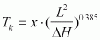
where T_K = time of concentration in h, L = running length = watershed - water-level gauge in km, DH = difference in level in m, x = calibration factor.
The discharge peak is determined by selecting a design precipitation of a certain duration TR and of the height h_N.

Fig. 13: Influence of the precipitation duration TR upon the discharge at constant concentration time TK

The discharge peak sought for the three possible cases is then:

(a) T_R = T_K
(b) T_R > T_K
(c) T_R < T_K

where T_R = duration of precipitation, h_N = height of precipitation, y = discharge coefficient, A_E0 = surface of catchment area, j = retardation coefficient (in approximation)

j = T_R/T_K

Here it must be taken into account that the intensity of precipitation in large catchment areas is smaller than in small catchment areas and that the intensity of rainfall decreases with the duration of rainfall. Detailed information is given in the literature [1] and [4].
In addition to these estimates, peak discharges can also be taken from specific peak discharge diagrams which are often available for regions for which comprehensive data exist (cf. Fig. 13).

Fig. 14: Idealized distribution of flow velocities v and suspended matter content CS in the vertical (y-direction) according to DVWK

1.3 Suspended matter and bed load

With the discharge each channel entrains solids in the form of suspended matter or bed load.

The suspended matter consists of small solid particles of various size held in suspension by buoyant forces in the water or by turbulence. In the water they are scarcely visible to the naked eye. Peak discharges of an intensive brown, for example, suggest a high solid matter concentration.

The bed load consists of solids such as fine sand, gravel with a small diameter of up to about 3 mm, or coarse material (gravel, stones of various size). The bed load is always transported on the river bottom.

The origin of the solids in the discharge of a channel can be attributed to a great number of causes; for example,

- surface erosion as a result of precipitation, chiefly in catchment areas with sparse vegetation cover,
- erosion in the river bed, in old branches, in reservoirs, and on foreshores, particularly in the case of peak discharges,
- pieces of plants and their decomposition products.

A particle can be transported in the discharge both as bed load and as suspended matter. An exact delimitation is not possible, as the influencesin particular the flow velocity - can be very different according to the discharge character.

Fig. 15: Distribution of suspended matter concentration of various soil types

The transport of the bed load is subject to the simple rule of thumb that the larger the particle to be transported and the greater its specific weight, the greater the tractive force of the water must be. High flow velocities (e.g. in the case of peak discharges) thus favour bed load transport.

The transport of suspended matter depends upon the settling velocity of the particle and thus upon the particle diameter, the particle form, the specific weight and the flow velocity.

According to Kresser, 1964 [15], the following relationship is valid as a rule of thumb for the determination of the limited particle diameter:

with g = 9.81 m/s, v_m = mean flow velocity in m/s.

The suspended matter concentration is unevenly distributed in the longitudinal section of the river. This is due to the variable vertical velocity distribution in the river section, which is shown in Fig. 14. Owing to the lower flow velocity, the idealized suspended matter content is higher in the vicinity of the river bottom than at the level of the surface of the water (cf. Fig. 14).

It also very much depends upon the type of particle, which can lead to other distributions of the suspended matter content. This can be seen from Fig. 15.

1.3.2 Stream-morphological influences upon solid matter transport

In the interplay between the tractive force of the water and the resistance of the bottom material, each stream is subject to changes. These are shown in simplified form in Fig. 16 for a longitudinal river section.

1. Erosion section
In the upper course of a river there is often no supply of solid matter from other inflows or solid matter from the surface erosion of the catchment area. Owing to the still low concentration of solid matters, the river is able to take up material, which results in erosion of the river bottom (depth erosion). This is also due to the flow velocities in the upper course which are higher due to the more pronounced slope.

A special case in the classification of this river section is latent erosion. Here, despite the lack of solid matter, the process of erosion has ceased, as the erodable bed material has already been transported downstream by continual scouring and the remaining coarse material forms a sort of protective layer.

2. Equilibrium sections
In the middle and lower course the supply of solid matter is meanwhile so great that the maximum transport capacity has been reached. Slight erosions are compensated by corresponding deposits, i.e. this river section is in equilibrium.

3. Accumulation sections {sedimentation)
In the lower course and the area of the estuary, the supply of solid matter may be so great that the transport capacity of the river is no longer sufficient and the excess solid matter is recognizable in the river bed as deposits (e.g. sand banks).

Fig. 16: Sequence of states in a longitudinal section of a river (qualitative)

In every river this theoretical sequence of erosion, equilibrium and accumulation sections can be observed several times in succession, this phenomenon being caused by the slope and local erosion bases. The construction of an intake structure may interfere with this river system.

Before an intake structure is planned, it is therefore necessary to obtain information on the solid matter transport upstream of and in the area of the intake structure so as to be able to estimate the influence of the structure upon the deposit of solid matter in front of it and the erosion behind it, and to determine the type of structure to be used.

Different sections of river can be distinguished by their appearance. This can be done according to the following criteria (source [6]):

1a) river section in a state of erosion:

- a small number of sand and gravel banks rapidly migrating downstream,
- steep banks, possibly steeper than would correspond to the natural angle of slope of the in-situ material,
- washing of the banks and slides in straight river sections,
- subsequent filing becoming necessary in order to secure the fill toes.

1b) river section in a state of latent erosion:

- steep slope (ravine section, gully),
- rocky bottom,
- bottom material coarser than on the banks,
- rock-slide material identifiable beyond any doubt as not belonging to the stream,
- bottom at the same level over a prolonged period in spite of steep slope and high flow velocities,
- no sand banks; gravel banks, if any, always in the same place.

2. river section in a state of equilibrium:

- slope remains constant over a prolonged time,
- bottom remains at the same level over a prolonged period,
- dimensions and form of the river cross-section do not progressively change (but changes over limited periods are possible during flooding),
- type and composition of the particles on the bottom and on the banks do not show fundamental differences,
- no washing of the banks in straight river sections,
- overflows always take place at more or less the same discharges,
- sand banks (if any) are stable and migrate downstream slowly, if at all.

3. river section in a state of accumulation:

- frequent, clearly visible gravel and sand banks often changing in form,
- bottom material finer than the material. On the banks,
- tendency to curve formation, formation of meanders,
- increase in the frequency of overflows and flooding,
- progressive alluvial deposits on the bottom and/or bank.

The influence of intake structures with and without damming upon the river upstream and downstream of the intake is described in detail in [6]. Methods for the quantitative estimate are also given there.

1.3.3 Measurement of amounts of suspended matter and bed load

The measurement of amounts of suspended matter and bed load is aimed at determining the solid matter content of a certain amount of water.

For the suspended matter measurement, indirect measuring methods are suitable which allow the suspended matter content (Cs) to be determined by drawing off a certain amount of water and filtering it, with a subsequent gravimetric determination of the filter residue. Like the discharge measurement, this measurement should, if possible, be carried out in various cross-sectional places of the river. Experience has shown that exact determination of the suspended matter content is possible only with multipoint measurements. The results always relate to the instantaneous discharge existing at the time of measurement, and therefore this discharge must be known. The following definitions are applicable:

- The suspended matter content is the mass of the suspended matter per unit of volume (Cs in mg/l or g/m³ ).
- By suspended matter transport msf in kg/s the suspended matter is meant which is transported through the cross-section in a certain unit of time.
- The suspended matter load msf is the suspended matter transport totalled for a certain unit of time (hour, day, month, etc.). The unit of time must be indicated.

The determination of the suspended matter content is of great importance. All terms always refer to the river section used for the suspended matter measurement.

For taking samples, numerous suspended matter measuring instruments are available which are placed in the water at the discharge measuring station with a cable crane installation, from a boat or from a bridge. These instruments can take water samples between 1 l and 5 I content. It is important that samples are taken from the various layers of the stream. The most suitable instrument is a wide-necked bottle with a content of 1 l.

A simple but relatively, inaccurate instrument for measuring suspended matter is a 51 to 10 I bucket whose content can be exactly read from marks, but this is suitable only for taking samples at the surface. The results thus obtained give only rough indications of the suspended matter content of a stream.

The measurement of the bed load is carried out with a bed load trap which consists of a wire mesh box opened towards the upstream side. As the bed load movement begins only at higher discharges, due to the then increased tractive force of the water, a bed load measurement is necessary only during peak discharges.

For the evaluation of the bed load measurement it is of particular importance to examine the particle composition by means of a screen analysis. Besides this analysis, a description of the bed load with respect to the kind of disposition, the kind of rock and particle size must be given.

As well as taking samples with the bed load trap, it is also possible at times of low discharge to take samples from deposits of sand and gravel banks after the top cover layer has been removed.

For a description of the bed load amounts in a river cross-section, the following definitions apply:

- bed load movement m_G in kg/(m · s) mass of bed load transported per unit of width and time;
- bed load transport m_G in kg/s mass of bed load transported through the cross-section in the unit of time;
- bed load m_Gf sum of the mass of bed load transported through the cross-section in a certain unit of time (e.g. month, year).